The difference between artificial intelligence and machine learning

Most people tend to use the terms artificial intelligence and machine learning interchangeably, especially people outside of the technology industry.

Artificial intelligence (AI) is simply a system that resembles human intelligence. Machine Learning (ML) is a system that is dependent on external data to learn. Thus, ML is a subset of AI.

Here is an example: suppose we want to build a program that looks at a photo to determine whether it contains a dog or not.

The AI approach is to hard-code what makes up a dog so the system knows. For example: does the animal have 4 legs, a tail, fur, and so on. The problem with this is that another animal sharing those features (a cat, for example) could be incorrectly identified as a dog.

With machine learning, we could feed the system lots of pictures of dogs and non-dogs and label what each one actually is. This is how the system learns. For complex recognition tasks, the ML approach is far superior to the rule-based AI approach.

There are three main types of machine learning training processes: Supervised, Unsupervised, and Reinforcement learning.

Supervised | You provide the correct answers for each piece of training data (from our example: dog, dog, not a dog, dog, etc).

Unsupervised | You don't give the system any answers. This is used primarily to find outlier data, for dimensionality reduction (i.e. reducing the complexity of training data while preserving its structure), or for clustering (grouping similar data points together).

Reinforcement | The system learns through trial and error. It receives a reward when it does something correctly and a penalty when it does something wrong, gradually learning the optimal behaviour over time.

Linear regression

Let's say we have a graph with many data points on it. We want to find the line of best fit — the one that gets as close as possible to all the data points.

This line can be represented by the following formula.

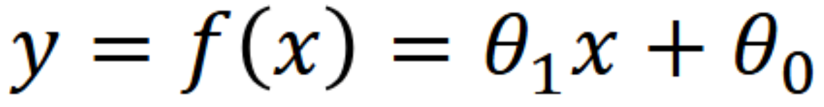
This formula is the same as y = mx + b, but we use theta notation because for more complex equations with multiple variables, it is easier to work with.

Now that we have a line, we can measure how far off the data points are from it. We use the following formula.

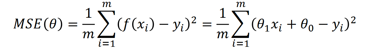
Measuring the difference between data points and a line is called a loss function. One of the most common types is the Mean Squared Error (MSE).

We take each predicted point on the line and subtract the real data value from it, giving us the error. We square this so that all errors are positive numbers. We repeat this for every data point, add them all together, and multiply by (1/m), where m is the total number of data points. This gives us the mean (average) error.

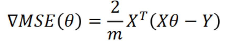
Ultimately, we want to minimise the mean squared error, so we need to adjust our line's slope (theta1) and/or y-intercept (theta0). A common technique for this is called gradient descent. This is the formula.

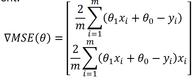
The result of this function is a vector with two values: the top value represents how much the loss changes with respect to theta0 (the y-intercept), and the bottom represents how much it changes with respect to theta1 (the slope). These are computed by taking the partial derivative of the loss function with respect to each parameter. The factor of 2/m arises naturally from differentiating the squared error term using the chain rule.

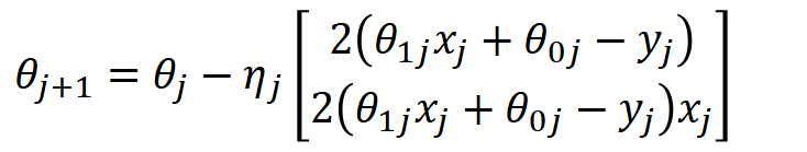
To actually update and improve our parameters, we use the following formula.

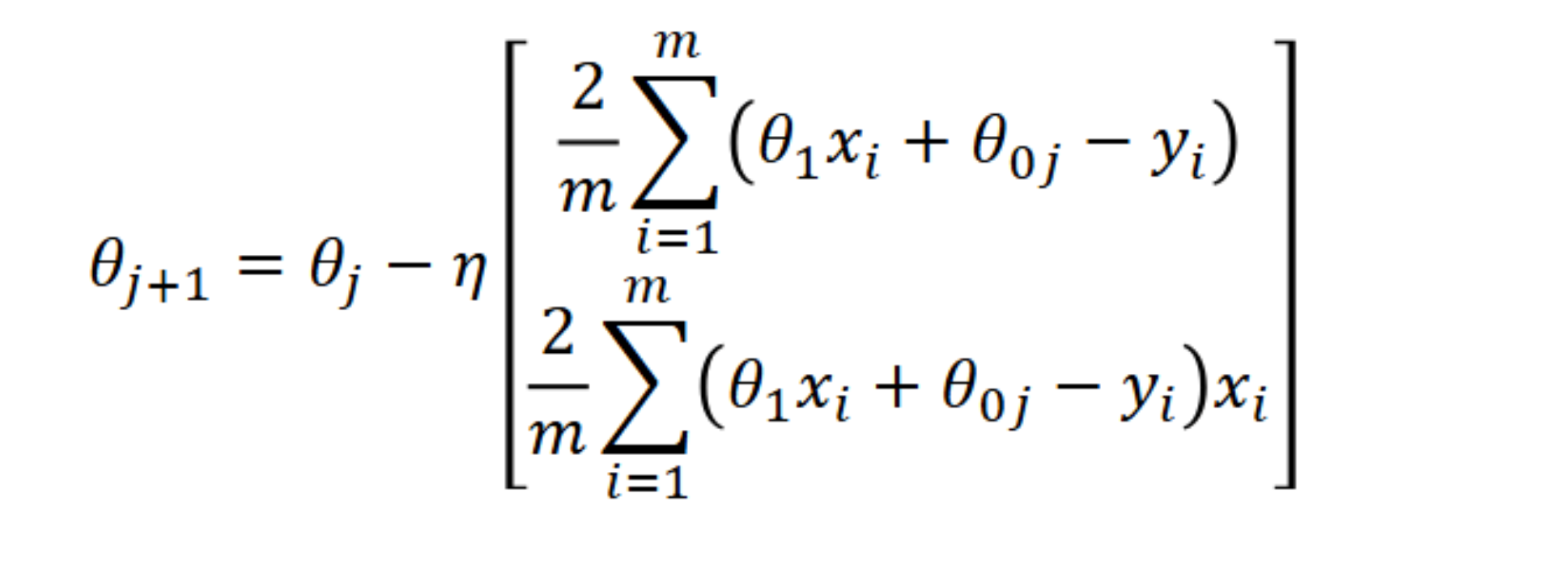
We multiply the gradient vector by a so-called learning rate that we set ourselves. This learning rate controls how drastically the parameters are adjusted at each step.

Think of it like throwing a basketball into a hoop. Throw too short and the ball doesn't reach. Overshoot and it goes too far. The learning rate needs to be just right — typically chosen through experimentation or based on how well the model is converging.

We then subtract this result from our current parameters thetaj (the current slope and y-intercept in vector form), giving us the updated parameters thetaj+1.

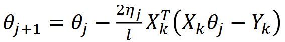
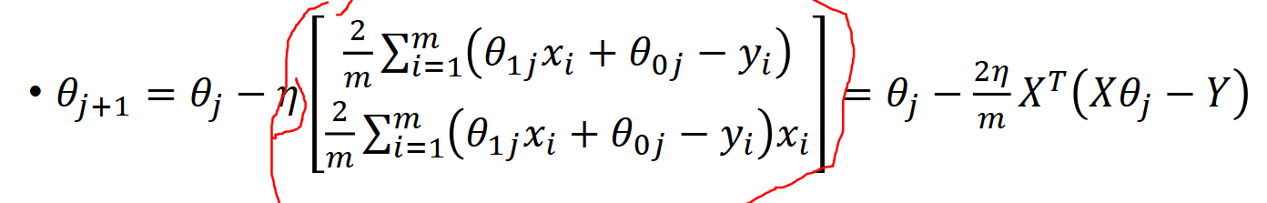
We can also represent this update rule in matrix form.

We compute the difference between the predicted values and the actual values in matrix form, then multiply by the transpose of X and (2/m). This is mathematically identical to the summation form but is much more efficient to compute in code.

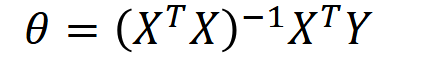
However, instead of using gradient descent to iteratively arrive at the optimal solution, we can get there in one step using the Normal Equation.

Types of gradient descent

Batch descent | The update rule is applied once using all the training data at the same time. This is accurate but becomes impractical with large datasets.

Stochastic descent | The update rule is applied using one random data point at a time, cycling through all data points in each epoch. It is computationally faster but produces a noisier, less stable path to the minimum.

Mini-batch descent | The update rule is applied using small random batches of data points (e.g. 5 out of 50) per iteration. This combines the efficiency of stochastic descent with the stability of batch descent, making it the most widely used approach in practice.